


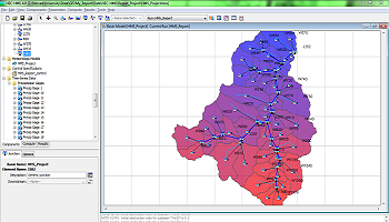
مثال پایه ای از مدل سازی نفوذ آب شور با SEAWAT و Flopy

SEAWAT یک مدل توسعه یافته توسط USGS برای شبیه سازی چگالی جریان آب زیرزمینی سه بعدی با انتقال شوری و گرما است. این نرم افزار بر اساس MODFLOW-2000 و MT3DMS است و در آخرین نسخه آن می تواند تغییرات ویسکوزیته را شبیه سازی کند و زمان اجرای سریع تر را فراهم کند. SEAWAT در Flopy، کتابخانه پایتون برای ساخت، اجرا و نمایش مدل MODFLOW اجرا می شود. این آموزش دارای جریان کاری کامل برای ایجاد و ارائه مثال پایه ای از ابزار سالین با SEAWAT و Flopy در یک نوت بوک Jupyter است.
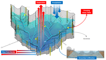
هندسه مدل
این مدل دارای 100 ستون، 50 لایه و 1 ردیف دارد. ابعاد مجموع در محور X، Y و Z به ترتیب 2، 1 و 1 متر است. یک چرخه تزریق در سمت چپ و یک هد ثابت در سمت راست وجود دارد.

داده های ورودی
شما می توانید فایل های ورودی برای آموزش را در اینجا دانلود کنید.
کد را در زیر مشاهده می کنید:
Import the required libraries
This tutorial requires some Python core libraries, Scipy libraries (numpy and matplotlib) as well as the Flopy library. Since we work on the interactive enviroment of Jupyter Notebook, we will use the Jupyter option to have inline output representation of the generated Matplotlib graphs. We will use some IPython widgets to create an interactive visualization of the model concentration distribution.
%matplotlib inline
import os
import sys
import numpy as np
import flopy
import flopy.utils.binaryfile as bf
import matplotlib.pyplot as plt
from matplotlib.colors import BoundaryNorm
from matplotlib.ticker import MaxNLocator
import ipywidgets as widgets
Create a basic MODFLOW model object
As well as any other model generated by Flopy, first we have to setup the model name and the working directory. We strongly recommend to follow the folder estructure provided on the "Input Files" of this tutorial.
# Create the basic MODFLOW model structure
modelname = 'model1a'
workspace = '../Model'
swt = flopy.seawat.Seawat(modelname, exe_name='../Exe/swt_v4x64.exe', model_ws=workspace)
print(swt.namefile)model1a.namDefine model dimensions, spatial discretization and hydraulic parameters
This model is almost a 2D models of 100 columns, 50 layers and 1 row. Total dimension in X, Y and Z axis are 2, 1 and 1 meter repectively. According to the Flopy input data procedure, there is only value or array for model_top (surface) and a list of elevations for every layer bottom elevation.
# Model dimensions
Lx = 2.
Ly = 1.
Lz = 1.
# Spatial discretization
nlay = 50
nrow = 1
ncol = 100
delr = Lx / ncol
delc = Ly
delv = Lz / nlay
# Elevation for model surface and layer bottom elevation
model_top = 1.
model_botm = np.linspace(model_top - delv, 0., nlay)
model_botmarray([0.98, 0.96, 0.94, 0.92, 0.9 , 0.88, 0.86, 0.84, 0.82, 0.8 , 0.78,
0.76, 0.74, 0.72, 0.7 , 0.68, 0.66, 0.64, 0.62, 0.6 , 0.58, 0.56,
0.54, 0.52, 0.5 , 0.48, 0.46, 0.44, 0.42, 0.4 , 0.38, 0.36, 0.34,
0.32, 0.3 , 0.28, 0.26, 0.24, 0.22, 0.2 , 0.18, 0.16, 0.14, 0.12,
0.1 , 0.08, 0.06, 0.04, 0.02, 0. ])# Another parameters
qinflow = 6.6E-5 # m3/s equiv to 5.702 m3/day
dmcoef = 6.6E-6 # m2/s equiv to 0.57024 m2/day Could also try 1.62925 as another case of the Henry problem
hk = 0.01 # m/s equivalent to 864m/dayDefinition of the flow packages for the SEAWAT model
In this part we define the packages related to groundwater flow on the SEAWAT model. First we define the DIS package that has the geometry as well as the simulation type (steady / transient). The model run on steady conditions on the head distribution, but transient on the saline distribution.
perlen = 86400 # 1 day in seconds

dis = flopy.modflow.ModflowDis(swt, nlay, nrow, ncol, nper=1, delr=delr,
                               delc=delc, laycbd=0, top=model_top,
                               botm=model_botm, perlen=perlen, nstp=15)
Then we define another SEAWAT packages as:
- the BAS package for setting the constant head cells,
- the LPF that defines the vertical / horizontal hydraulic conductivity,
- the PCG packages that solves the model matrix
- the OC packages for the output record
# Variables for the BAS package
ibound = np.ones((nlay, nrow, ncol), dtype=np.int32)
ibound[:, :, -1] = -1
bas = flopy.modflow.ModflowBas(swt, ibound, 0)

# Add LPF package to the MODFLOW model
lpf = flopy.modflow.ModflowLpf(swt, hk=hk, vka=hk, ipakcb=53)

# Add PCG Package to the MODFLOW model
pcg = flopy.modflow.ModflowPcg(swt, hclose=1.e-8)

# Add OC package to the MODFLOW model
oc = flopy.modflow.ModflowOc(swt,
                             stress_period_data={(0, 0): ['save head', 'save budget']},
                             compact=True)
Definition of the flow and transport packages for the SEAWAT model
A well is created with the WEL package and defined as a source of fresh water with concentration of 0. The left boundary is defined as sea water with concentration of 35. The well inflow is distributed over the model layers.
# Create WEL and SSM data
itype = flopy.mt3d.Mt3dSsm.itype_dict()
wel_data = {}
ssm_data = {}
wel_sp1 = []
ssm_sp1 = []
for k in range(nlay):
    wel_sp1.append([k, 0, 0, qinflow / nlay])
    ssm_sp1.append([k, 0, 0, 0., itype['WEL']])
    ssm_sp1.append([k, 0, ncol - 1, 35., itype['BAS6']])
wel_data[0] = wel_sp1
ssm_data[0] = ssm_sp1
wel = flopy.modflow.ModflowWel(swt, stress_period_data=wel_data, ipakcb=53)
Setup of the MT3DMS models and the SEAWAT variable density flow package
According with the SEAWAT setup the paramaters for the transport model. Values variable density flow package of Seawat are also declared.
# Create the basic MT3DMS model structure
btn = flopy.mt3d.Mt3dBtn(swt, nprs=-5, prsity=0.35, sconc=35., ifmtcn=0,
                         chkmas=False, nprobs=10, nprmas=10, dt0=300)
adv = flopy.mt3d.Mt3dAdv(swt, mixelm=0)
dsp = flopy.mt3d.Mt3dDsp(swt, al=0., trpt=1., trpv=1., dmcoef=dmcoef)
gcg = flopy.mt3d.Mt3dGcg(swt, iter1=500, mxiter=1, isolve=1, cclose=1e-7)
ssm = flopy.mt3d.Mt3dSsm(swt, stress_period_data=ssm_data)

# Create the SEAWAT model structure
vdf = flopy.seawat.SeawatVdf(swt, iwtable=0, densemin=0, densemax=0,
                             denseref=1000., denseslp=0.7143, firstdt=1e-3)
Write files of the SEAWAT model and run simulation
Write the .nam file and the files declared on the .nam file. Then runs the simulation and shows the simulation information on the screen
# Write the input files
swt.write_input()
swt.run_model()
FloPy is using the following executable to run the model: ../Exe/swt_v4x64.exe
SEAWAT Version 4
U.S. GEOLOGICAL SURVEY MODULAR FINITE-DIFFERENCE GROUND-WATER FLOW MODEL
Version 4.00.05 10/19/2012
Incorporated MODFLOW Version: 1.18.01 06/20/2008
Incorporated MT3DMS Version: 5.20 10/30/2006
This program is public domain and is released on the
condition that neither the U.S. Geological Survey nor
the United States Government may be held liable for any
damages resulting from their authorized or unauthorized
use.
Using NAME file: model1a.nam
Run start date and time (yyyy/mm/dd hh:mm:ss): 2019/02/18 10:30:57
STRESS PERIOD NO. 1
STRESS PERIOD 1 TIME STEP 1 FROM TIME = 0.0000 TO 5760.0
Transport Step: 1 Step Size: 300.0 Total Elapsed Time: 300.00
Outer Iter. 1 Inner Iter. 1: Max. DC = 0.4179 [K,I,J] 50 1 1
Outer Iter. 1 Inner Iter. 2: Max. DC = 0.3685 [K,I,J] 1 1 2
Outer Iter. 1 Inner Iter. 3: Max. DC = 0.2005 [K,I,J] 1 1 3
Outer Iter. 1 Inner Iter. 4: Max. DC = 0.2249 [K,I,J] 49 1 3
.....
Run end date and time (yyyy/mm/dd hh:mm:ss): 2019/02/18 10:31:02
Elapsed run time: 5.310 Seconds
Normal termination of SEAWAT
(True, [])Model results post-processing
This tutorial has three representations of the flow and transport model with SEAWAT:
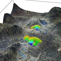
- The first representation is a flow direction vector over the concentrations at the end of the model
- Second representation is the head distribution on the model extension
- Third representation is a interactive graph of concentration development along the model time steps.
1. Flow directions and concentrations
# Load data
ucnobj = bf.UcnFile('../Model/MT3D001.UCN', model=swt)
times = ucnobj.get_times()
concentration = ucnobj.get_data(totim=times[-1])
cbbobj = bf.CellBudgetFile('../Model/model1a.cbc')
times = cbbobj.get_times()
qx = cbbobj.get_data(text='flow right face', totim=times[-1])[0]
qz = cbbobj.get_data(text='flow lower face', totim=times[-1])[0]

# Average flows to cell centers
qx_avg = np.empty(qx.shape, dtype=qx.dtype)
qx_avg[:, :, 1:] = 0.5 * (qx[:, :, 0:ncol-1] + qx[:, :, 1:ncol])
qx_avg[:, :, 0] = 0.5 * qx[:, :, 0]
qz_avg = np.empty(qz.shape, dtype=qz.dtype)
qz_avg[1:, :, :] = 0.5 * (qz[0:nlay-1, :, :] + qz[1:nlay, :, :])
qz_avg[0, :, :] = 0.5 * qz[0, :, :]
# parameters for the colorbar
levels = MaxNLocator(nbins=15).tick_values(concentration.min(), concentration.max())
cmap = plt.get_cmap('PiYG')
norm = BoundaryNorm(levels, ncolors=cmap.N, clip=True)# Make the plot
fig = plt.figure(figsize=(20, 10))
ax = fig.add_subplot(1, 1, 1, aspect='equal')
im = ax.imshow(concentration[:, 0, :], interpolation='nearest',
extent=(0, Lx, 0, Lz))
fig.colorbar(im, ax=ax, fraction=0.05, label="Concentration (g/l)")
y, x, z = dis.get_node_coordinates()
X, Z = np.meshgrid(x, z[:, 0, 0])
iskip = 3
ax.quiver(X[::iskip, ::iskip], Z[::iskip, ::iskip],
qx_avg[::iskip, 0, ::iskip]*1E5, -qz_avg[::iskip, 0, ::iskip]*1E5,
color='w', scale=3, headwidth=3, headlength=2,
headaxislength=2, width=0.0025)
ax.set_title('Flow Direction and Concentration')
plt.savefig('../Output/ConcentrationDistribution.png')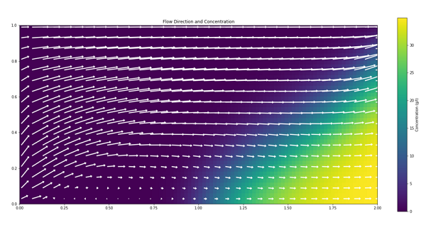
2. Head distribution on model extension
# Extract the heads
fname = '../Model/model1a.hds'
headobj = bf.HeadFile(fname)
times = headobj.get_times()
head = headobj.get_data(totim=times[-1])
head[0:3,0,0:3]
array([[-0.00049478, -0.00062826, -0.00076412],
[-0.00049201, -0.00062547, -0.00076129],
[-0.00048649, -0.0006199 , -0.00075567]], dtype=float32)levels = MaxNLocator(nbins=15).tick_values(head.min(), head.max())
cmap = plt.get_cmap('Blues')
norm = BoundaryNorm(levels, ncolors=cmap.N, clip=True)# Make a simple head plot
fig = plt.figure(figsize=(20, 10))
ax = fig.add_subplot(1, 1, 1, aspect='equal')
im = ax.imshow(head[:, 0, :], interpolation='nearest',
extent=(0, Lx, 0, Lz))
fig.colorbar(im, ax=ax, fraction=0.05, label="Head (m)")
ax.set_title('Simulated Heads')
plt.savefig('../Output/HeadDistribution.png')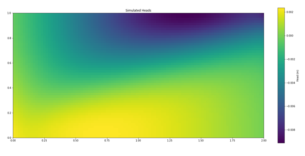
3. Interactive representation of concentration development
times = np.asarray(ucnobj.get_times())
times[:5]
array([1500., 3000., 4500., 5760., 7260.], dtype=float32)def plotConcentration(time):
# Load data
ucnobj = bf.UcnFile('../Model/MT3D001.UCN', model=swt)
concentration = ucnobj.get_data(totim=time)
# For colormap
levels = MaxNLocator(nbins=15).tick_values(concentration.min(), concentration.max())
cmap = plt.get_cmap('PiYG')
norm = BoundaryNorm(levels, ncolors=cmap.N, clip=True)
#Figure definition
fig = plt.figure(figsize=(20, 10))
ax = fig.add_subplot(1, 1, 1, aspect='equal')
im = ax.imshow(concentration[:, 0, :], interpolation='nearest',
extent=(0, Lx, 0, Lz))
cbaxes = fig.add_axes([0.05, 0.15, 0.02, 0.7])
fig.colorbar(im, ax=ax, fraction=0.05, label="Concentration (g/l)", cax = cbaxes)# create a model interactive representation
widgets.interact(plotConcentration, time=widgets.SelectionSlider(options=times, value=times[0], disabled=False))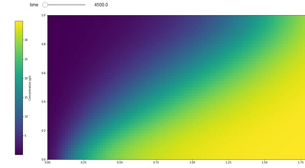

مدیر سایت: بهزاد سرهادی کارشناس ارشد مهندسی آب
شناسه تلگرام مدیر سایت: SubBasin@
نشانی ایمیل: behzadsarhadi@gmail.com
(سوالات تخصصی را در گروه تلگرام ارسال کنید)
_______________________________________________________
پروژه تخصصی در لینکدین


 در منابع آب


نظرات (۰)