


مدلسازی آب های زیر زمینی منطقه ای با MODFLOW و Flopy

مدل سازی منطقه ای آب های زیرزمینی یک وظیفه مهم در مدیریت آب استراتژیک است که شامل تمام کاربران، فعالیت ها و اکوسیستم های مربوطه و استفاده پایدار از شرایط فعلی و آینده است. برخی از ملاحظات خاص در مورد مدلسازی منطقه ای با توجه به تقسیم بندی اولیه و فضایی وجود دارد؛ یک مدل منطقه ای در نظر گرفته نشده است که پاسخ منطقه آبخوان را برای منطقه مشخص تعیین کند، در عوض شامل ارزیابی جریان آب های زیرزمینی منطقه و اندازه گیری شارژ، تخلیه و سایر فرآیندهای موجود در تعادل آب است.
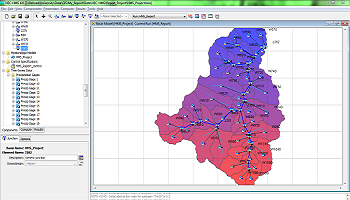
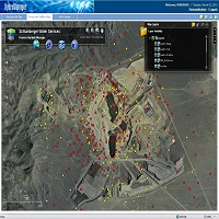
این آموزش نسخه Flopy از نمونه عددی از حوضه Angascancha با MODFLOW و Model Muse است که شما می توانید در مطالب مشابه پیدا کنید. مثال در حالت پایدار است و با حل کننده NWT حل شده است. نمایندگی مدل خروجی تحت ابزار Flopy / Matplotlib و همچنین بعضی از کد های Python برای ایجاد فایل های VTU و Style در Paraview انجام شده است.
فایل های ورودی
شما می توانید فایل های ورودی این آموزش را در این لینک دانلود کنید.
Python code
This is the described Python code for this tutorial:
Import the required libraries
This tutorial requires some Python core libraries, Scipy libraries (numpy and matplotlib) as well as the Flopy library. For the management and data extraction from raster files we use the GDAL library.
import flopy
import os
import flopy.utils.binaryfile as bf
import numpy as np
from osgeo import gdal
import matplotlib.pyplot as plt
Create a basic MODFLOW model object
As well as any other model generated by Flopy, first we have to setup the model name and the working directory. We strongly recommend to follow the folder/file estructure provided on the "Input Files" of this tutorial. Based on the complex geometry and the differences among layers elevations and layer thickness, the NWT solver has been applied to the model.
modelname = "model1"
modelpath = "../Model/"
#Modflow Nwt
mf1 = flopy.modflow.Modflow(modelname, exe_name="../Exe/MODFLOW-NWT_64.exe", version="mfnwt",model_ws=modelpath)
nwt = flopy.modflow.ModflowNwt(mf1 ,maxiterout=150,linmeth=2)
Open and read raster files
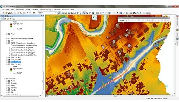
In this part we will use the GDAL library to open the rasters of elevation and boundary conditions and get their geotransformation parameters. The tutorial requires that the raster resolution is the same as the grid resolution. Raster bands are read as Numpy arrays and inserted to the model as model top.
#Raster paths
demPath ="../Rst/DEM_200.tif"
crPath = "../Rst/CR.tif"

#Open files
demDs =gdal.Open(demPath)
crDs = gdal.Open(crPath)
geot = crDs.GetGeoTransform() #Xmin, deltax, ?, ymax, ?, delta y

geot
(613882.5068, 200.0, 0.0, 8375404.9524, 0.0, -200.0)# Get data as arrays
demData = demDs.GetRasterBand(1).ReadAsArray()
crData = crDs.GetRasterBand(1).ReadAsArray()
# Get statistics
stats = demDs.GetRasterBand(1).GetStatistics(0,1)
stats[3396.0, 4873.0, 4243.0958193041, 287.90182492684]Spatial discretization
Since this tutorial deals with a regional scale, the differences in elevation on the area of study can be more than a hundred meters or more than a thousand meters if we deal with andean basins. The hydrogeological conceptualization for this tutorial is the definition of two upper thin layers (Layer1 and Layer1_2) and thicker layers below.
#Elevation of layers
Layer1 = demData - 7.5
Layer1_2 = demData - 15
Layer2 = (demData - 3000)*0.8 + 3000
Layer3 = (demData - 3000)*0.5 + 3000
Layer4 = (demData>0)*3000
Column and row number and dimension come from the raster attributes
#Boundaries for Dis = Create discretization object, spatial/temporal discretization
ztop = demData
zbot = [Layer1, Layer1_2, Layer2, Layer3, Layer4]
nlay = 5
nrow = demDs.RasterYSize
ncol = demDs.RasterXSize
delr = geot[1]
delc = abs(geot[5])
Definition of the flow packages for the MODFLOW model
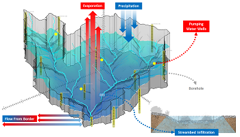
In this part we define the packages related to groundwater flow on the MODFLOW model. First we define the DIS package that has the geometry as well as the simulation type (steady / transient). The model run on steady conditions.
dis = flopy.modflow.ModflowDis(mf1, nlay,nrow,ncol,delr=delr,delc=delc,top=ztop,botm=zbot,itmuni=1)Then we define another MODEL packages. Some boundary conditions are setup from raster valures, while other packages use constant value. These are the required packages for the simulation:
- the BAS package for setting the constant head cells and inactive cells,
- the UPW that defines the vertical / horizontal hydraulic conductivity,
- the RCH package that applies rechage from precipitation
- the EVT package for the simulation of groundwater consumption from roots
- the DRN package for the groundwater discharge to the channel network
- the OC packages for the output record
# Variables for the BAS package
iboundData = np.zeros(demData.shape, dtype=np.int32)
iboundData[crData > 0 ] = 1
bas = flopy.modflow.ModflowBas(mf1,ibound=iboundData,strt=ztop, hnoflo=-2.0E+020)
# Array of hydraulic heads per layer
hk = [1E-4, 1E-5, 1E-7, 1E-8, 1E-9]
# Add UPW package to the MODFLOW model
upw = flopy.modflow.ModflowUpw(mf1, laytyp = [1,1,1,1,0], hk = hk)#Add the recharge package (RCH) to the MODFLOW model
rch = np.ones((nrow, ncol), dtype=np.float32) * 0.120/365/86400
rch_data = {0: rch}
rch = flopy.modflow.ModflowRch(mf1, nrchop=3, rech =rch_data)#Add the evapotranspiration package (EVT) to the MODFLOW model
evtr = np.ones((nrow, ncol), dtype=np.float32) * 1/365/86400
evtr_data = {0: evtr}
evt = flopy.modflow.ModflowEvt(mf1,nevtop=1,surf=ztop,evtr=evtr_data, exdp=0.5)#Add the drain package (DRN) to the MODFLOW model
river = np.zeros(demData.shape, dtype=np.int32)
river[crData == 3 ] = 1
list = []
for i in range(river.shape[0]):
for q in range(river.shape[1]):
if river[i,q] == 1:
list.append([0,i,q,ztop[i,q],0.001]) #layer,row,column,elevation(float),conductanceee
rivDrn = {0:list}
drn = flopy.modflow.ModflowDrn(mf1, stress_period_data=rivDrn)# Add OC package to the MODFLOW model
oc = flopy.modflow.ModflowOc(mf1) #ihedfm= 1, iddnfm=1Write files of the MODFLOW model and run simulation
Write the .nam file and the files declared on the .nam file. Then runs the simulation and shows the simulation information on the screen
#Write input files -> write file with extensions
mf1.write_input()

#run model -> gives the solution
mf1.run_model()
FloPy is using the following executable to run the model: ../Exe/MODFLOW-NWT_64.exe
MODFLOW-NWT-SWR1
U.S. GEOLOGICAL SURVEY MODULAR FINITE-DIFFERENCE GROUNDWATER-FLOW MODEL
WITH NEWTON FORMULATION
Version 1.1.4 4/01/2018
BASED ON MODFLOW-2005 Version 1.12.0 02/03/2017
SWR1 Version 1.04.0 09/15/2016
Using NAME file: model1.nam
Run start date and time (yyyy/mm/dd hh:mm:ss): 2019/02/22 10:19:24
Solving: Stress period: 1 Time step: 1 Groundwater-Flow Eqn.
Run end date and time (yyyy/mm/dd hh:mm:ss): 2019/02/22 10:20:04
Elapsed run time: 39.475 Seconds
Normal termination of simulation
(True, [])Model results post-processing
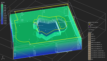
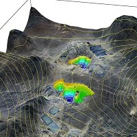
This tutorial has some model features and output representation done with Flopy and Matplotlib. Another 3D representation on the VTK format is performed on another notebook from this tutorial
#Import model
ml = flopy.modflow.Modflow.load('../Model/model1.nam')
Model grid representation
# First step is to set up the plot
fig = plt.figure(figsize=(15, 15))
ax = fig.add_subplot(1, 1, 1, aspect='equal')

# Next we create an instance of the ModelMap class
modelmap = flopy.plot.ModelMap(sr=ml.dis.sr)

# Then we can use the plot_grid() method to draw the grid
# The return value for this function is a matplotlib LineCollection object,
# which could be manipulated (or used) later if necessary.
linecollection = modelmap.plot_grid(linewidth=0.4)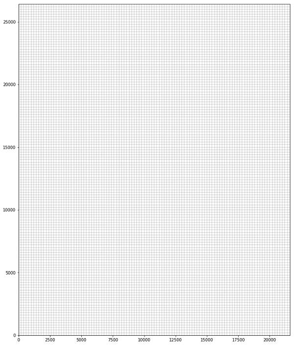
Cross section of model grid representation
fig = plt.figure(figsize=(15, 6))
ax = fig.add_subplot(1, 1, 1)
# Next we create an instance of the ModelCrossSection class
#modelxsect = flopy.plot.ModelCrossSection(model=ml, line={'Column': 5})
modelxsect = flopy.plot.ModelCrossSection(model=ml, line={'Row': 99})

# Then we can use the plot_grid() method to draw the grid
# The return value for this function is a matplotlib LineCollection object,
# which could be manipulated (or used) later if necessary.
linecollection = modelxsect.plot_grid(linewidth=0.4)
t = ax.set_title('Column 6 Cross-Section - Model Grid')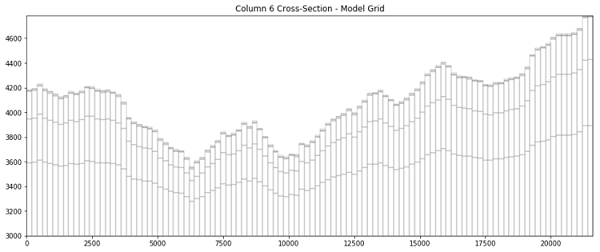
Active/inactive cells on model extension
fig = plt.figure(figsize=(15, 15))
ax = fig.add_subplot(1, 1, 1, aspect='equal')
modelmap = flopy.plot.ModelMap(model=ml, rotation=0)
quadmesh = modelmap.plot_ibound(color_noflow='cyan')
linecollection = modelmap.plot_grid(linewidth=0.4)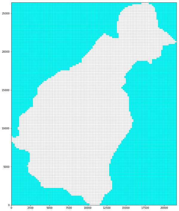
Cross sections of active/inactive cells
fig = plt.figure(figsize=(15, 6))
ax = fig.add_subplot(1, 1, 1)
modelxsect = flopy.plot.ModelCrossSection(model=ml, line={'Column': 5})
patches = modelxsect.plot_ibound(color_noflow='cyan')
linecollection = modelxsect.plot_grid(linewidth=0.4)
t = ax.set_title('Column 6 Cross-Section with IBOUND Boundary Conditions')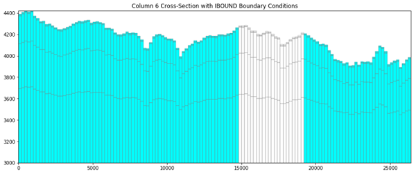
Channel network as drain (DRN) package
fig = plt.figure(figsize=(15, 15))
ax = fig.add_subplot(1, 1, 1, aspect='equal')
modelmap = flopy.plot.ModelMap(model=ml, rotation=-14)
quadmesh = modelmap.plot_ibound(color_noflow='cyan')
quadmesh = modelmap.plot_bc('DRN', color='blue')
linecollection = modelmap.plot_grid(linewidth=0.4)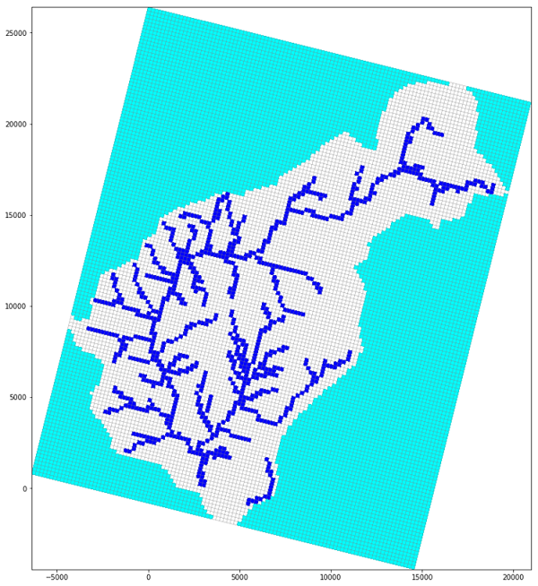
Model grid and heads representation
fname = os.path.join(modelpath, 'model1.hds')
hdobj = flopy.utils.HeadFile(fname)
head = hdobj.get_data()

fig = plt.figure(figsize=(30, 30))
ax = fig.add_subplot(1, 2, 1, aspect='equal')
modelmap = flopy.plot.ModelMap(model=ml, rotation=-14)
#quadmesh = modelmap.plot_ibound()
quadmesh = modelmap.plot_array(head, masked_values=[-2.e+20], alpha=0.8)
linecollection = modelmap.plot_grid(linewidth=0.2)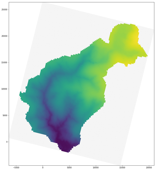

برای یافتن تمامی مطالب مرتبط با این مطلب در سایت از جستجوی سایت در حاشیه سمت راست و بالای صفجه استفاده فرمایید.

ورود به بخش آموزش های متنی GMS


دانلود آخرین نسخه نرم افزار GMS

دریافت لایسنس ارزیابی (14 روزه)


مدیر سایت: بهزاد سرهادی کارشناس ارشد مهندسی آب
شناسه تلگرام مدیر سایت: SubBasin@
نشانی ایمیل: behzadsarhadi@gmail.com
(سوالات تخصصی را در گروه تلگرام ارسال کنید)
_______________________________________________________
پروژه تخصصی در لینکدین


 در منابع آب


نظرات (۰)